Show the code
library(tidyverse)
library(tidycensus)Population pyramids are graphs that show the age distribution of a population. They’re usually divided by sex and start with the youngest age group on the bottom and the oldest on the top.
Population pyramids are used for all types of populations, from humans to mice. Their overall shape tells us information about the study population to the demographer or population ecologist, from birth rates to age-dependency rate to predictions of the future of that population (aka population forecasts), from predictions in the US 40 years ago that Social Security would run out of money in the 2020’s to concerns about Japan’s and China’s aging populations.
So, how do we make a population pyramid? First, let’s load the libraries.
library(tidyverse)
library(tidycensus)Tidycensus loads US Census data in tibble form, compatible with the Tidyverse and various mapping packages. You can get more information on using it here. Before you can download data, however, you need an API key from the Census Bureau that you can sign up for here.
census_api_key("a4808358dcde1ac0bac19a6e7686329bcee6ff7a", install = TRUE, overwrite = TRUE)[1] "a4808358dcde1ac0bac19a6e7686329bcee6ff7a"options(tigris_use_cache = TRUE)Once you get an API key, you enter it using the census_api_key() function. Also note that I set the cache option as “TRUE” so RStudio won’t have to make multiple calls for data.
Tidycensus specializes in data from the decennial censuses (i.e. 2000, 2010, 2020) and from the American Community Survey (ACS) taken each year between decennial censuses. The ACS are available in 1-year form from each year or as 5-year averages. When you start, a big roadblock to downloading the data you want is simply that you don’t know the names of the data files. That is solved with a call to get all of the available data.
v21 <- load_variables(2021, "acs5", cache = TRUE)

head(v21)
# A tibble: 6 × 4
name label concept geography
<chr> <chr> <chr> <chr>
1 B01001A_001 Estimate!!Total: SEX BY AGE (WHI… tract
2 B01001A_002 Estimate!!Total:!!Male: SEX BY AGE (WHI… tract
3 B01001A_003 Estimate!!Total:!!Male:!!Under 5 years SEX BY AGE (WHI… tract
4 B01001A_004 Estimate!!Total:!!Male:!!5 to 9 years SEX BY AGE (WHI… tract
5 B01001A_005 Estimate!!Total:!!Male:!!10 to 14 years SEX BY AGE (WHI… tract
6 B01001A_006 Estimate!!Total:!!Male:!!15 to 17 years SEX BY AGE (WHI… tract In this example, I called for the variable names available in the 2021 5-year-average ACS. Note I had to specify the year and which survey I wanted. If you wanted the yearly ACS, just specify “acs1” instead. I’d have used the 2022 survey but it isn’t available yet. Now to call for the specific table and do some data wrangling.
# Get population data by metro area, then narrow it down to a specific metro area and get rid of three summary lines

Dayton_metro_pop_pyramid <- get_acs(geography = "cbsa",
                   table = "B01001",
                   year = 2021,
                   survey = "acs5"
                   ) %>%
        filter(NAME == "Dayton-Kettering, OH Metro Area") %>%
        filter(!row_number() %in% c(1, 2, 26))
head(Dayton_metro_pop_pyramid)
# A tibble: 6 × 5
GEOID NAME variable estimate moe
<chr> <chr> <chr> <dbl> <dbl>
1 19430 Dayton-Kettering, OH Metro Area B01001_003 24684 131
2 19430 Dayton-Kettering, OH Metro Area B01001_004 24946 1000
3 19430 Dayton-Kettering, OH Metro Area B01001_005 26465 977
4 19430 Dayton-Kettering, OH Metro Area B01001_006 16103 99
5 19430 Dayton-Kettering, OH Metro Area B01001_007 11431 239
6 19430 Dayton-Kettering, OH Metro Area B01001_008 6233 669Looking at the data, it’s not quite ready for analysis yet. So I cleaned it up further with the following steps
# Add sex and lower age limits in machine-readable form

Dayton_metro_pop_pyramid$Sex <- rep(c("male", "female"), each = 23)

Dayton_metro_pop_pyramid$Lower_Age <- rep(c(0, 5, 10, 15, 18, 20, 21, 22, 25, 30, 35, 40, 45, 50, 55, 60, 62, 65, 67, 70, 75, 80, 85), length = 46)

# Get uniform 5 years groups and make the Male population estimates negative. Round the 18, 21, 22, 62, and 67 Age groups down to the nearest multiple of 5 and then add their estimated population to the others of that multiple.

Dayton_metro_pop_pyramid <- Dayton_metro_pop_pyramid %>%
        mutate(estimate = case_when(
                Sex == "male" ~ -estimate,
                TRUE ~ estimate
                ),
               Lower_Age = Lower_Age - Lower_Age %% 5
        ) %>%
        mutate(Lower_Age = as_factor(Lower_Age)) %>%
        select(Lower_Age, Sex, estimate) %>%
        group_by(Sex, Lower_Age) %>%
        summarize(estimate = sum(estimate))

head(Dayton_metro_pop_pyramid)
# A tibble: 6 × 3
# Groups: Sex [1]
Sex Lower_Age estimate
<chr> <fct> <dbl>
1 female 0 23322
2 female 5 23225
3 female 10 25521
4 female 15 26516
5 female 20 26543
6 female 25 27610Now, finally, the data is in the correct form for making a population pyramid. I used the ggplot2 package to make the graph.
Dayton_age_pyramid <- ggplot(Dayton_metro_pop_pyramid,
                             aes(x = estimate,
                                 y = Lower_Age,
                                 fill = Sex)) +
        theme_classic() +
        geom_col() +
        labs(title = "Population Pyramid, Dayton, OH, metro area",
             x = "Population",
             y = "Age bracket")

Dayton_age_pyramid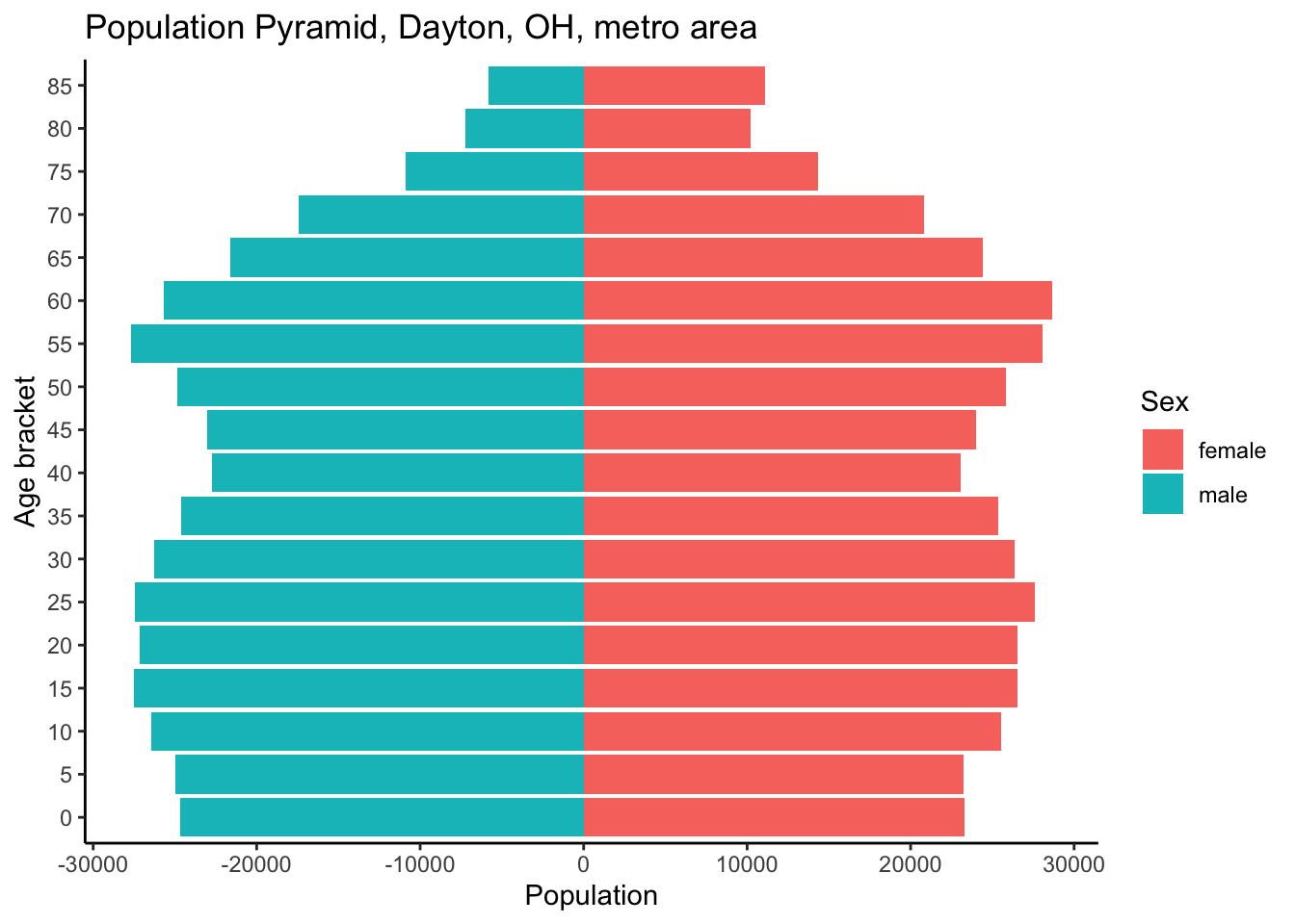
Looking at the population of the Dayton, Ohio, metro area, we see a fairly uniform shape signifying a stable population size. One concern for this area in the future is the smaller bars of under-10 years old cohorts, signifying a possible population decrease in the future or at best slow population growth.
And there you have it. A population pyramid created in R using US Census data. Hope this helps.
Notes, suggestions, remarks? Feel free to leave a comment below.